NN training
Given that the zero-loss peak background cannot be evaluated from first principles, in this work we deploy supervised machine learning combined with Monte Carlo methods to construct a neural network parameterisation of the ZLP. Within this approach, one can faithfully model the ZLP dependence on both the electron energy loss and on the local specimen thickness. Our approach, first presented in [Roest et al., 2021], is here extended to model the thickness dependence and to the simultaneous interpretation of the \(\mathcal{O}(10^4)\) spectra that constitute a typical EELS-SI. One key advantage is the robust estimate of the uncertainties associated to the ZLP modelling and subtraction procedures using the Monte Carlo replica method [Collaboration et al., 2007].
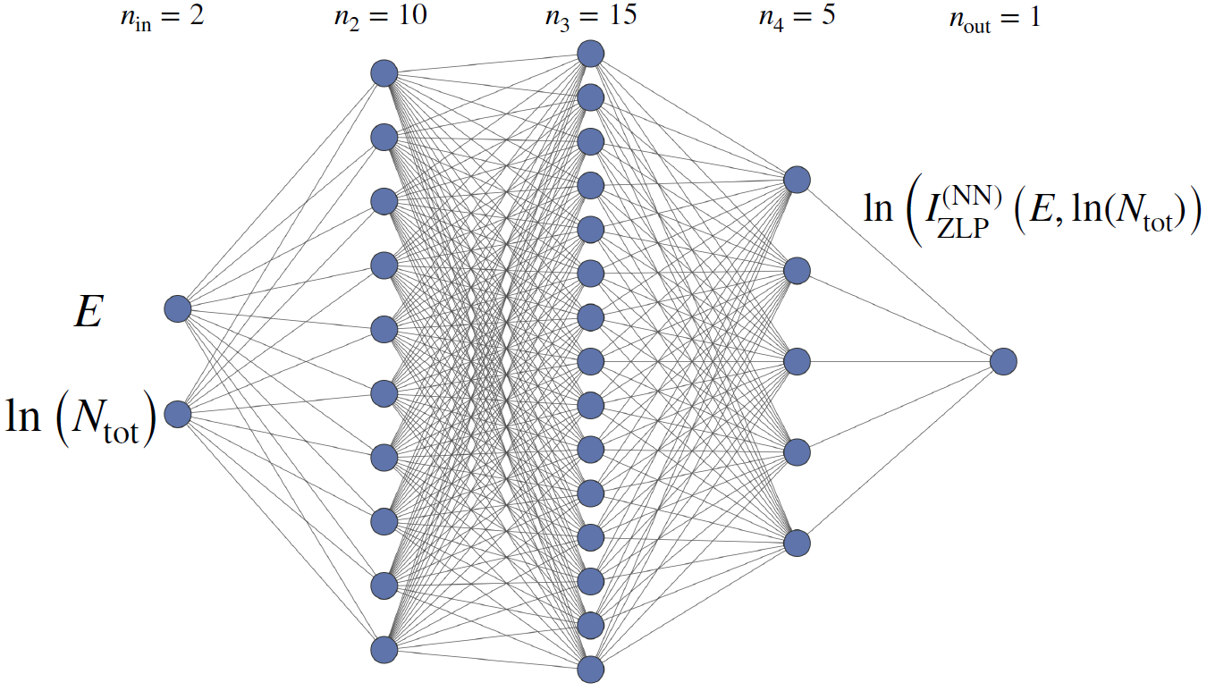
Fig. 4 The neural network architecture parametrising the ZLP. The input neurons are the energy loss \(E\) and the logarithm of the integrated intensity \(N_{\rm tot}\) , while the output neuron is the (logarithm of the) model prediction for the ZLP intensity.
The neural network architecture adopted in this work is displayed in Fig. 4. It contains two input variables, namely the energy loss \(E\) and the logarithm of the integrated intensity \(\ln\left( N_{\rm tot}\right)\), the latter providing a proxy for the thickness \(t\). Both \(E\) and \(\ln\left( N_{\rm tot}\right)\) are preprocessed and rescaled to lie between 0.1 and 0.9 before given as input to the network. Three hidden layers contain 10, 15, and 5 neurons respectively. The activation state of the output neuron in the last layer, \(\xi^{(n_L)}_1\), is then related to the intensity of the ZLP as
where an exponential function is chosen to facilitate the learning, given that the EELS intensities in the training dataset can vary by orders of magnitude. Sigmoid activation functions are adopted for all layers except for a ReLU in the final layer, to guarantee a positive-definite output of the network and hence of the predicted intensity.
The training of this neural network model for the ZLP is carried out as follows. Assume that the input SI has been classified into \(K\) clusters following the procedure of App.~ref{sec:processing-SI}. The members of each cluster exhibit a similar value of the local thickness. Then one selects at random a representative spectrum from each cluster,
each one characterised by a different total integrated intensity evaluated from Eq. (3),
such that \((i_k,j_k)\) belongs to the \(k\)-th cluster. To ensure that the neural network model accounts only for the energy loss \(E\) dependence in the region where the ZLP dominates the recorded spectra, we remove from the training dataset those bins with \(E \ge E_{{\rm I},k}\) with \(E_{{\rm I},k}\) being a model hyperparameter [Roest et al., 2021] which varies in each thickness cluster. The cost function \(C_{\rm ZLP}\) used to train the NN model is then
where the total number of energy loss bins that enter the calculation is the sum of bins in each individual spectrum, \(n_{E} = \sum_{k=1}^K n_E^{(k)} \, .\) The denominator of Eq. (7) is given by \(\sigma_k \left( E_{\ell_k}\right)\), which represents the variance within the \(k\)-th cluster for a given value of the energy loss \(E_{\ell_k}\). This variance is evaluated as the size of the 68% confidence level (CL) interval of the intensities associated to the \(k\)-th cluster for a given value of \(E_{\ell_k}\).
For such a random choice of representative cluster spectra, Eq. (6), the parameters (weights and thresholds) of the neural network model are obtained from the minimisationof (7) until a suitable convergence criterion is achieved. Here this training is carried out using stochastic gradient descent (SGD) as implemented in the {tt PyTorch} library [Paszke et al., 2019], specifically by means of the ADAM minimiser. The optimal training length is determined by means of the look-back cross-validation stopping. In this method, the training data is divided \(80\%/20\%\) into training and validation subsets, with the best training point given by the absolute minimum of the validation cost function \(C_{\rm ZLP}^{(\rm val)}\) evaluated over a sufficiently large number of iterations.
In order to estimate and propagate uncertainties associated to the ZLP parametrisation and subtraction procedure, here we adopt a variant of the Monte Carlo replica method [Roest et al., 2021] benefiting from the high statistics (large number of pixels) provided by an EELS-SI. The starting point is selecting \(N_{\rm rep}\simeq \mathcal{O}\left( 5000\right)\) subsets of spectra such as the one in Eq. (6) containing one representative of each of the \(K\) clusters considered. One denotes this subset of spectra as a Monte Carlo (MC) replica, and we denote the collection of replicas by
where now the superindices \((i_{m,k},j_{m,k})\) indicate a specific spectrum from the \(k\)-th cluster that has been assigned to the \(m\)-th replica. Given that these replicas are selected at random, they provide a representation of the underlying probability density in the space of EELS spectra, e.g. those spectra closer to the cluster mean will be represented more frequently in the replica distribution.
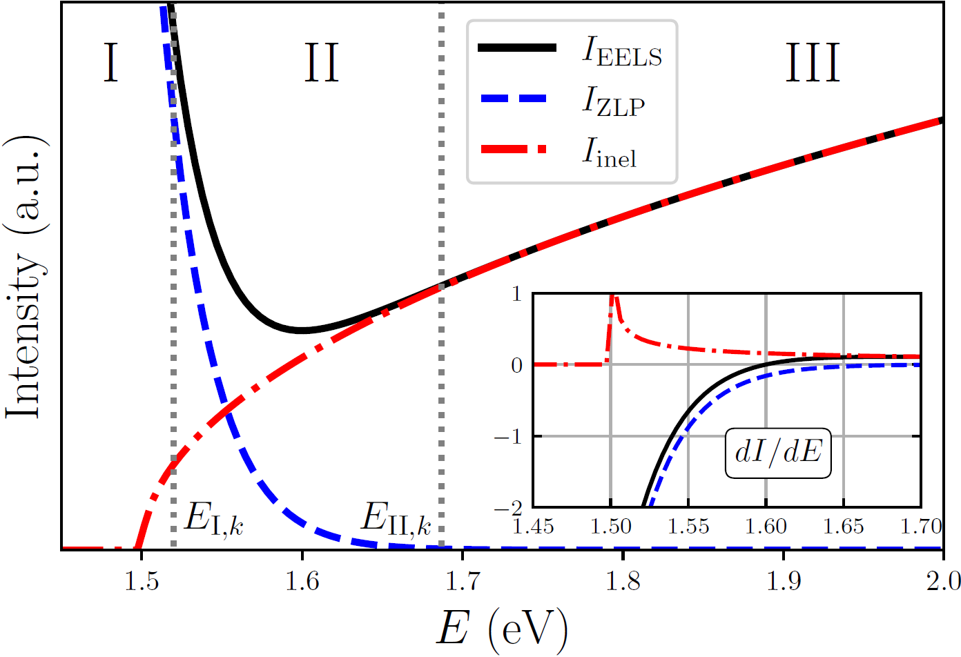
Fig. 5 Schematic representation of the ZLP and inelastic scattering contributions adding up to the total EELS intensity within a toy simulation. We indicate the values of the hyperparameters \(E_{{\rm I},k}\) and \(E_{{\rm II},k}\) for such configuration: the neural network model for the ZLP is trained on the data corresponding to region I (hence \(E\le E_{{\rm I},k}\) ), while the behaviour in region II is determined purely from model predictions. The inset displays the first derivative of each of the three curves.
By training now a separate model to each of the \(N_{\rm rep}\) replicas, one ends up with another Monte Carlo representation, now of the probability density in the space of ZLP parametrisations. This is done by replacing the cost function (9)
by
and then performing the model training separately for each individual replica. Note that the denominator of the cost function Eq. (10) is independent of the replica. The resulting Monte Carlo distribution of ZLP models, indicated by
makes possible subtracting the ZLP from the measured EELS spectra following the matching procedure described in [Roest et al., 2021] and hence isolating the inelastic contribution in each pixel,
The variance of \(I_{\rm inel}^{(i,j)}(E)\) over the MC replica sample estimates the uncertainties associated to the ZLP subtraction procedure. By means of these MC samplings of the probability distributions associated to the ZLP and inelastic components of the recorded spectra, one can evaluate the relevant derived quantities with a faithful error estimate. Note that in our approach error propagation is realised without the need to resort to any approximation, e.g. linear error analysis.
One important benefit of Eq. (10) is that the machine learning model training can be carried out fully in parallel, rather than sequentially, for each replica. Hence our approach is most efficiently implemented when running on a computer cluster with a large number of CPU (or GPU) nodes, since this configuration maximally exploits the parallelization flexibility of the Monte Carlo replica method.
As mentioned above, the cluster-dependent hyperparameters \(E_{{\rm I},k}\) ensure that the model is trained only in the energy loss data region where ZLP dominates total intensity. This is illustrated by the scheme of Fig. 5, showing a toy simulation of the ZLP and inelastic scattering contributions adding up to the total recorded EELS intensity. The neural network model for the ZLP is then trained on the data corresponding to region I and region III, while region II is obtained entirely from model predictions. To determine the values of \(E_{{\rm I},k}\), we determine the point of highest curvature between the Full Width at Half Maximum on the log values of the signal and the local minimum. From there, \(E_{{\rm I},k}\) is shifted to the desired value. This ensures \(E_{{\rm I},k}\) is always located near the ZLP in case the sample signal is unable to overcome the signal of the ZLP tail + noise floor (this could occure in aloof areas of the spectral image).
The second model hyperparameter, denoted by \(E_{{\rm II},k}\) in Fig. 5, indicates the region for which the ZLP can be considered as fully negligible. Hence in this region III we impose that \(I_{\rm ZLP}(E)\to 0\) by means of the Lagrange multiplier method. This condition fixes the model behaviour in the large energy loss limit, which otherwise would remain unconstrained. Since the ZLP is known to be a steeply-falling function, \(E_{{\rm II},k}\) should not chosen not too far from \(E_{{\rm I},k}\) to avoid an excessive interpolation region. We determine \(E_{{\rm II},k}\) by fitting a log10 function through the point of highest curvature and the local minimum. The point where this fit crosses with a single count is where we put \(E_{{\rm II},k}\), with shift it for fine tuning. This approach puts \(E_{{\rm II},k}\) in a similar location as the signal-to-noise method presented in [Roest et al., 2021].
To ensure our models are monotomically decreasing in the region of \(E_{{\rm I},k}\) and \(E_{{\rm II},k\), we add a penalty term to the cost function \(\lambda\), improving the output of our neural network,
Finally, we mention that the model hyperparameters \(E_{{\rm I},k}\) and \(E_{{\rm II},k}\) could eventually be determined by means of an automated hyper-optimisation procedure as proposed in [Ball et al., 2022], hence further reducing the need for human-specific input in the whole procedure.