Pooling and clustering

Let us consider a two-dimensional region of the analysed specimen with dimensions \(L_x\times L_y\) where EEL spectra are recorded for \(n_p=n_x \times n_y\) pixels. Then the information contained within an EELS-SI may be expressed as

(1)\[I^{(i,j)}_{\rm EELS}(E_\ell) \,, \quad i=1,\ldots, n_x\,, \quad j=1,\ldots, n_y\,, \quad \ell=1,\ldots, n_E \, ,\]

With each spectra constructed as

(2)\[I^{(i,j)}_{\rm EELS}(E_\ell) = I^{(i,j)}_{\rm ZLP}(E_\ell) + I^{(i,j)}_{\rm inel}(E_\ell) \, ,\]

where \(I^{(i,j)}_{\rm EELS}(E_\ell)\) indicates the recorded total electron energy loss intensity for an energy loss \(E_\ell\) for a location in the specimen (pixel) labelled by \((i,j)\), and \(n_E\) is the number of bins that compose each spectrum. \(I^{(i,j)}_{\rm ZLP}(E_\ell)\) indicates the ZLP contributions and \(I^{(i,j)}_{\rm inel}(E_\ell)\) the inelastic scattering contribution. The spatial resolution of the EELS-SI in the \(x\) and \(y\) directions is usually taken to be the same, implying that

\[\Delta x = \Delta y \simeq \frac{L_x}{n_x} = \frac{L_y}{n_y} \, .\]

For the specimens analysed in this work we have \(n_p=\mathcal{O}(10^4)\) spectra corresponding to a spatial resolution of \(\Delta x \simeq 10\) nm. On the one hand, a higher spatial resolution is important to allow the identification and characterisation of localised features within a nanomaterial, such as structural defects, phase boundaries, surfaces or edges. On the other hand, if the resolution \(\Delta x\) becomes too small the individual spectra become noisy due to limited statistics. Hence, the optimal spatial resolution can be determined from a compromise between these two considerations.

In general it is not known what the optimal spatial resolution should be prior to the EELS-TEM inspection and analysis of a specimen. Therefore, it is convenient to record the spectral image with a high spatial resolution and then, if required, combine subsequently the information on neighbouring pixels by means of a procedure known as pooling or sliding-window averaging. The idea underlying pooling is that one carries out the following replacement for the entries of the EELS spectral image listed in Eq. (1):

\[I^{(i,j)}_{\rm EELS}(E_\ell)\quad \to I^{(i,j)}_{\rm EELS}(E_\ell)\Big|_{\rm pooled} =\frac{1}{N^{(i,j)}_{\rm pool}}\sum_{|i'-i|\le d} \sum_{|j'-j|\le d}\left( \omega_{|i'-i|,|j'-j|} \times I^{(i',j')}_{\rm EELS}(E_\ell)\right) \, ,\]

where \(d\) indicates the pooling range, \(\omega_{|i'-i|,|j'-j|}\) is a weight factor, and the pooling normalisation is determined by the sum of the relevant weights,

\[N^{(i,j)}_{\rm pool} = \sum_{|i'-i|\le d} \sum_{|j'-j|\le d} \omega_{|i'-i|,|j'-j|} \, .\]

By increasing the pooling range \(d\), one combines the local information from a higher number of spectra and thus reduces statistical fluctuations, at the price of some loss on the spatial resolution of the measurement. For instance, \(d=3/2\) averages the information contained on a \(3\times 3\) square centered on the pixel \((i,j)\). Given that there is no unique choice for the pooling parameters, one has to verify that the interpretation of the information contained on the spectral images does not depend sensitively on their value. In this work, we consider uniform weights, \(\omega_{|i'-i|,|j'-j|}=1\), but other options such as Gaussian weights

\[\omega_{|i'-i|,|j'-j|} = \exp\left( - \frac{(i-i')^2}{2d^2} - \frac{(j-j')^2}{2d^2} \right) \, ,\]

with \(\sigma^2=d^2\) as variance are straightforward to implement in {scsmall EELSfitter}. The outcome of this procedure is a a modified spectral map with the same structure as Eq. (1) but now with pooled entries. In this work we typically use \(d=3\) to tame statistical fluctuations on the recorded spectra.

As indicated by Eq. (2), the total EELS intensity recorded for each pixel of the SI receives contributions from both inelastic scatterings and from the ZLP, where the latter must be subtracted before one can carry out the theoretical interpretation of the low-loss region measurements. Given that the ZLP arises from elastic scatterings with the atoms of the specimen, and that the likelihood of these scatterings increases with the thickness, its contribution will depend sensitively with the local thickness of the specimen. Hence, before one trains the deep-learning model of the ZLP it is necessary to first group individual spectra as a function of their thickness. In this work this is achieved by means of unsupervised machine learning, specifically with the \(K\)-means clustering algorithm. Since the actual calculation of the thickness has as prerequisite the ZLP determination, see Eq. (26), it is suitable to use instead the total integrated intensity as a proxy for the local thickness for the clustering procedure. That is, we cluster spectra as a function of

(3)\[N^{(i,j)}_{\rm tot} \equiv \int_{-\infty}^{\infty} dE\, I_{\rm EELS}^{(i,j)}(E) = \int_{-\infty}^{\infty} dE\,\left( I^{(i,j)}_{\rm ZLP}(E) + I^{(i,j)}_{\rm inel}(E) \right) = N^{(i,j)}_0 + N^{(i,j)}_{\rm inel} \, ,\]

which coincides with the sum of the ZLP and inelastic scattering normalisation factors. Eq. (3) is inversely proportional to the local thickness \(t\) and therefore represents a suitable replacement in the clustering algorithm. In practice, the integration in Eq. (3) is restricted to the measured region in energy loss.

The starting point of \(K\)-means clustering is a dataset composed by \(n_p=n_x\times n_y\) points,

\[\ln\left( N^{(r)}_{\rm tot}\right) \,,\quad r=1,\ldots , n_p\,, \qquad r=i+(n_y-1)j \, ,\]

which we want to group into \(K\) separate clusters \(T_k\), whose means are given by

\[\ln \left( \widetilde{N}^{(k)}\right) \,,\quad k=1,\ldots, K\,.\]

The cluster means represent the main features of the \(k\)-th cluster to which the data points will be assigned in the procedure. Clustering on the logarithm of \(N^{(r)}_{\rm tot}\) rather than on its absolute value is found to be more efficient, given that depending on the specimen location the integrated intensity will vary by orders of magnitude.

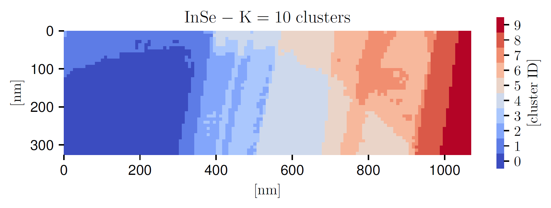
Fig. 2 The outcome of the \(K\) -means clustering procedure applied to the InSe specimen, where each color represents one of the \(K=10\) thickness clusters. It can be compared with the thickness map of Fig. 3 .

In \(K\)-means clustering, the determination of the cluster means and data point assignments follows from the minimisation of a cost function. This is defined in terms of a distance in specimen thickness space, given by

(4)\[C_{\rm Kmeans}\left( {\boldsymbol N}_{\rm tot}, {\boldsymbol T}\right) = \sum_{r=1}^{n_p}\sum_{k=1}^{K} d_{rk}\left| \ln\left( \frac{\widetilde{N}^{(k)}}{N^{(r)}_{\rm tot}}\right) \right|^p \, ,\]

with \(d_{rk}\) being a binary assignment variable, equal to 1 if \(r\) belongs to cluster \(k\) (\(d_{rk}=1\) for \(r\in T_k\)) and zero otherwise, and with the exponent satisfying \(p> 0\). Here we adopt \(p=1/2\), which reduces the weight of eventual outliers in the calculation of the cluster means, and we verify that results are stable if \(p=1\) is used instead. Furthermore, since clustering is exclusive, one needs to impose the following sum rule

\[\sum_{k=1}^K d_{rk}=1 \, ,\quad \forall\,r \, .\]

The minimisation of Eq. (4) results in a cluster assignment such that the internal variance is minimised and is carried out by means of a semi-analytical algorithm. This algorithm is iterated until a convergence criterion is achieved, e.g. when the change in the cost function between two iterations is below some threshold. Note that, as opposed to supervised learning, here is it not possible to overfit and eventually one is guaranteed to find the solution that leads to the absolute minimum of the cost function. The end result of the clustering process is that now we can label the information contained in the (pooled) spectral image (for \(r=i+(n_y-1)j\)) as follows

(5)\[\begin{split}I^{(i,j)}_{{\rm EELS},k}(E_\ell) = \begin{cases} I^{(r)}_{\rm EELS}(E_\ell)\quad {\rm if} \quad r\in T_k \\ 0 \quad {\rm otherwise} \end{cases} \,, \quad k=1,\dots, K\, .\end{split}\]

This cluster assignment makes possible training the ZLP deep-learning model across the complete specimen recorded in the SI accounting for the (potentially large) variations in the local thickness.

The number of clusters \(K\) is a free parameter that needs to be fixed taking into consideration how rapidly the local thickness varies within a given specimen. We note that \(K\) cannot be too high, else it will not be possible to sample a sufficiently large number of representative spectra from each cluster to construct the prior probability distributions, as required for the Monte Carlo method used in this work. We find that \(K=10\) for the InSe and \(K=5\) for the \(WS_2\) specimens are suitable choices. Fig. 2 displays the outcome of the \(K\)-means clustering procedure applied to the InSe specimen, where each color represents one of the \(K=10\) thickness clusters. It can be compared with the corresponding thickness map in Fig. 3; the qualitative agreement further confirms that the total integrated intensity in each pixel \(N_{\rm tot}^{(i,j)}\) represents a suitable proxy for the local specimen thickness.

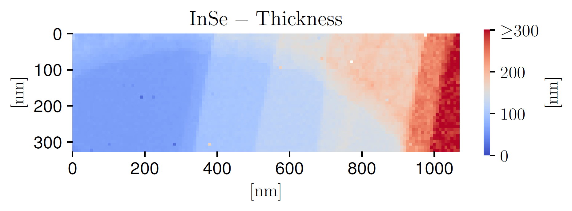
Fig. 3 The thickness map corresponding to the InSe SI.