![]()
EELSfitter tutorial
In this tutorial, we are going to train a model of the zero-loss peak (ZLP) background of polytopic WS\(_2\) nanoflowers. Individiual spectra are first classified as a function of the local thickness with \(K\)-means clustering before serving as input to a feedforward neural network.
The ZLP models can be used to obtain a ZLP-subtracted spectral image (SI), which in turn gives access to the dielectric function through the Kramers-Krönig analysis. One can also find the bandgap energy from the subtracted spectrum.
Installing EELSfitter
To install EELSFitter, if not done already, one should run the following command.
[ ]:
!pip install EELSFitter
This is a necessary step if one chooses to run from google colab. This step can be skipped if one is running locally and EELSFitter has already been installed.
Loading the SI
First of all, let us import the EELSFitter package:
[1]:
import os
import numpy as np
import wget

import EELSFitter as ef
from EELSFitter.plotting.zlp import plot_zlp_per_pixel, plot_zlp_per_cluster
from EELSFitter.plotting.heatmaps import plot_heatmap

from matplotlib import rc

# If you want to use LaTeX for typesetting, use this.
rc('font', **{'family': 'sans-serif', 'sans-serif': ['Computer Modern'], 'size': 12})
rc('text', usetex=True)
Next, we download and load the spectral image and specify the location where we would like to store our output, such as plots.
[2]:
dm4_url='https://github.com/LHCfitNikhef/EELSfitter/blob/documentation/tutorials/area03-eels-SI-aligned.dm4?raw=true'
wget.download(dm4_url)
[2]:
'area03-eels-SI-aligned.dm4'
[2]:
path_to_image = "area03-eels-SI-aligned.dm4"
im = ef.SpectralImage.load_data(path_to_image)
im.output_path = os.path.join(os.getcwd(), 'output\\')

if not os.path.exists(im.output_path):
    os.mkdir(im.output_path)
In case the metadata doesn’t contain the correct information (as with this data file), run the following cell to put the correct beam energy, collection angle and convergence angle.
[3]:
im.beam_energy = 200            # KeV
im.collection_angle = 67.2      # mrad
im.convergence_angle = 67.2     # mrad
The below specifies some of our plot settings:
[4]:
# Colormap
cmap="coolwarm"

# Tick settings
npix_xtick = 99.25 / (im.y_axis[-1]/len(im.y_axis))
npix_ytick = 99.25 / (im.y_axis[-1]/len(im.y_axis))
sig_ticks = 3
tick_int = True
cb_scale = 0.8

# Title and save location settings
title_specimen = r'$\rm{WS_2\;nanoflower\;}$'
save_title_specimen = 'WS2_nanoflower_flake'
save_loc = im.output_path
Visualising the SI
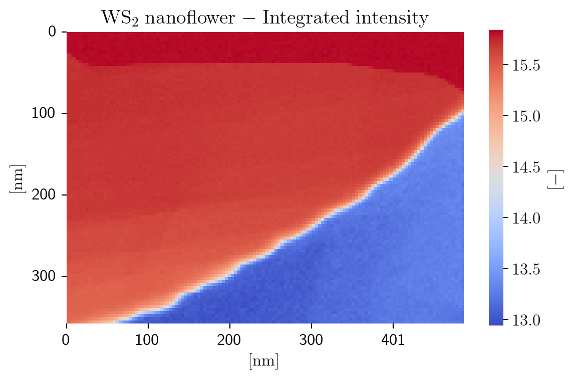
With the spectral image loaded, we can take a first look at what our image actually looks like. We decide to produce a heatmap of the integrated intensity, which is a measure of the local thickness.
[5]:
intensity = np.log(np.sum(im.data, axis=2))
save_as = os.path.join(save_loc, "Integrated_Intensity")
fig = plot_heatmap(im, intensity,
                   title=title_specimen + r'$\rm{-\;Integrated\;intensity\;}$',
                   cbar_kws={'label': r'$\rm{[-]\;}$','shrink':cb_scale}, cmap=cmap,
                   sig_ticks=sig_ticks, npix_xtick=npix_xtick, npix_ytick=npix_ytick, tick_int=tick_int,
                   save_as=save_as)
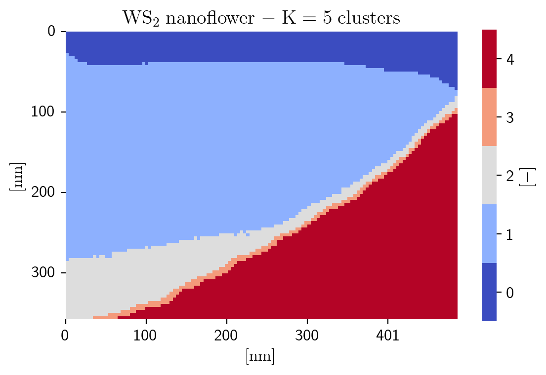
Clustering
Since the ZLP intensity depends strongly on the local thickness of the specimen, first of all we group individual spectra as a function of their thickness by means of unsupervised machine learning, specifically by means of the K-means clustering algorithm:
[6]:
n_clusters = 5
based_on = 'log_zlp'
seed = 12345678
im.cluster(n_clusters=n_clusters, based_on=based_on, seed=seed)
Seed: 12345678 finished after 11 iterations and has cost: 284.1100204608507
Seed: 12345678 has the lowest cost
# of spectra per cluster is [1419 6002 1193  209 3209]
[7]:
fig = plot_heatmap(im, im.cluster_labels,
                   title=title_specimen +  r'$\rm{-\;K=%d\;clusters\;}$' % n_clusters,
                   cbar_kws={'label': r'$\rm{[-]\;}$','shrink':cb_scale}, cmap=cmap, discrete_colormap=True,
                   sig_ticks=sig_ticks, npix_xtick=npix_xtick, npix_ytick=npix_ytick, tick_int=tick_int,
                   save_as=save_loc + save_title_specimen + '_Clustered')
Training of the ZLP
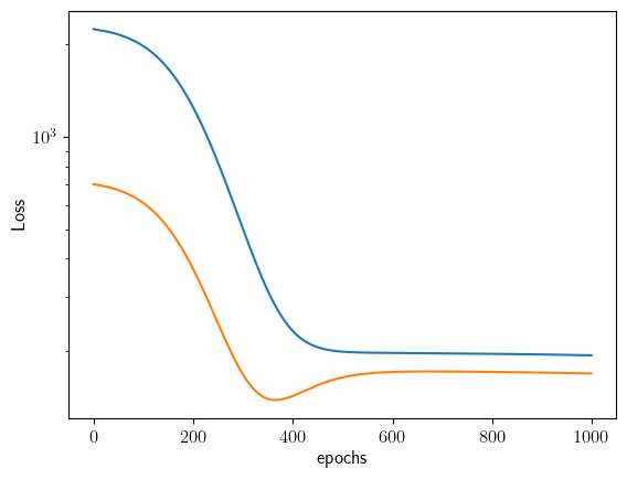
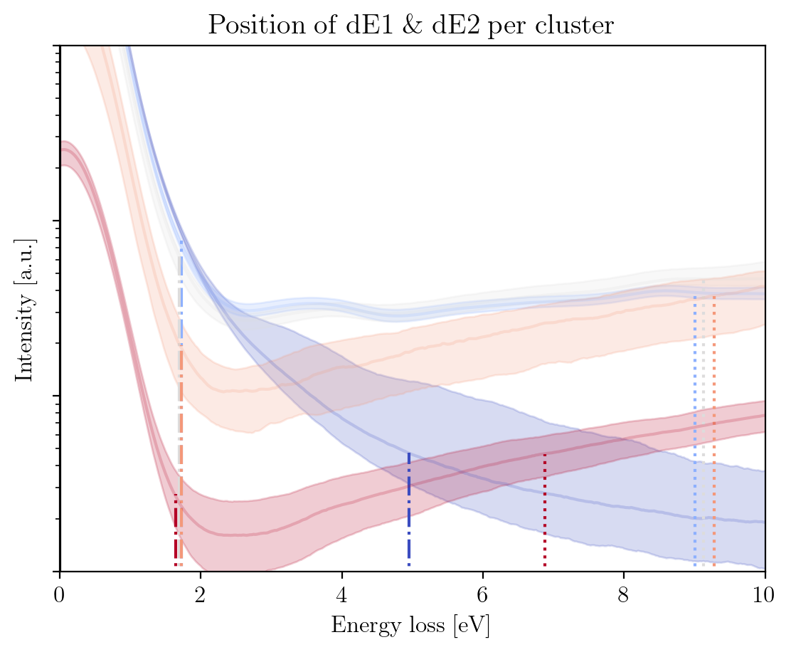
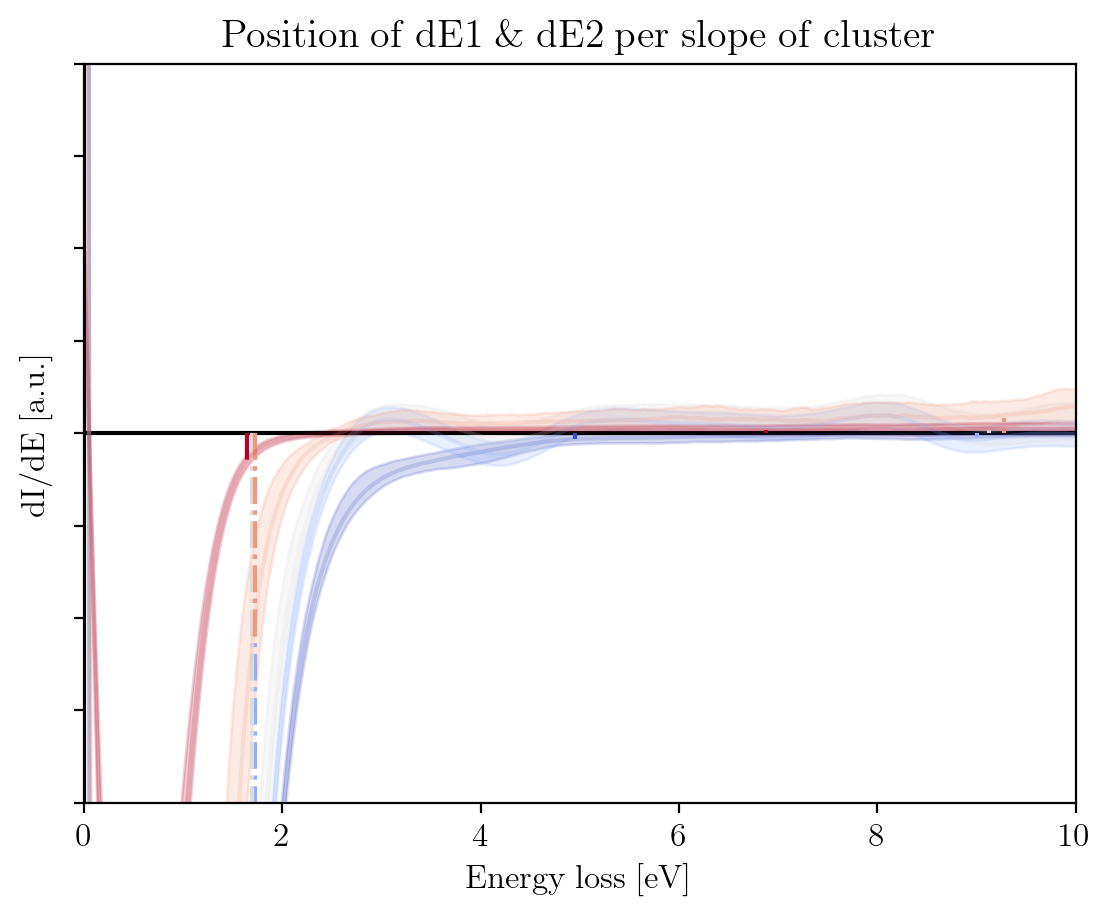
The ZLP can be trained with the following lines of code. It produces a couple of plots: 1. The raw signal per cluster, including the position of the hyperparamter \(E_I\) 2. The slow of the raw signal per cluster 3. The value of the loss per epoch on both training and validation set
The more replicas one uses to train the ZLP, the more accurate the model becomes.
[8]:
n_replica = 1                   # number of replicas
n_epochs = 1000                 # number of epochs
regularisation_constant = 1.    # Penalty term to prevent models from going up in region II, set to 0 to disable. This will increase training time significantly if enabled.
display_step = 200              # show training report after display_step steps

# Choose to shift the hyperparameters a bit
shift_dE1 = 1.
shift_dE2 = 1.

signal_type = 'EELS'

path_to_models = os.path.join(im.output_path, "models") # where to store the trained models
if not os.path.exists(path_to_models):
    os.mkdir(path_to_models)

im.train_zlp_models(n_clusters=n_clusters,
                    seed=seed,
                    based_on=based_on,
                    n_replica=n_replica,
                    n_epochs=n_epochs,
                    shift_de1=shift_dE1,
                    shift_de2=shift_dE2,
                    regularisation_constant=regularisation_constant,
                    display_step=display_step,
                    path_to_models=path_to_models,
                    signal_type=signal_type)

fig1 = im.train_zlps.plot_hp_cluster(title=r'$\rm{Position\;of\;dE1\;\&\;dE2\;per\;cluster\;}$',
                                     xlabel=r'$\rm{Energy\;loss\;[eV]\;}$',
                                     ylabel=r'$\rm{Intensity\;[a.u.]\;}$',
                                     xlim=[0, 10],
                                     ylim=[10, 1e4],
                                     yscale='log')

fig2 = im.train_zlps.plot_hp_cluster_slope(title=r'$\rm{Position\;of\;dE1\;\&\;dE2\;per\;slope\;of\;cluster\;}$',
                                           xlabel=r'$\rm{Energy\;loss\;[eV]\;}$',
                                           ylabel=r'$\rm{dI/dE\;[a.u.]\;}$',
                                           xlim=[0, 10],
                                           ylim=[-1e3, 1e3])
Seed: 12345678 finished after 11 iterations and has cost: 284.1100204608507
Seed: 12345678 has the lowest cost
# of spectra per cluster is [1419 6002 1193  209 3209]
preparing hyperparameters!
No crossing found in gain region cluster 0, finding minimum of absolute of dydx
No crossing found in gain region cluster 1, finding minimum of absolute of dydx
No crossing found in gain region cluster 2, finding minimum of absolute of dydx
No crossing found in gain region cluster 3, finding minimum of absolute of dydx
Log10 fit cluster  0  does not cross a single count, setting intersect index to second eaxis index
Log10 fit cluster  1  does not cross a single count, setting intersect index to second eaxis index
Log10 fit cluster  2  does not cross a single count, setting intersect index to second eaxis index
Log10 fit cluster  3  does not cross a single count, setting intersect index to second eaxis index
Log10 fit cluster  4  does not cross a single count, setting intersect index to second eaxis index
dE1: [4.95  1.725 1.7   1.725 1.65 ]
dE2: [44.25   9.     9.125  9.275  6.875]
I'm saving hyperparameters.txt so hang on...
clusters centroids=[13.85190143 13.50152474 13.04813684 11.50411317  9.21495881] size (5,)
dE1=[4.95000007 1.72500003 1.70000003 1.72500003 1.65000002] has size (5,)
dE2=[44.25000066  9.00000013  9.12500014  9.27500014  6.8750001 ] has size (5,)
FWHM=[0.72500001 0.72500001 0.72500001 0.77500001 0.80000001] has size (5,)
Saved hyperparameters.txt!
Hyperparameters prepared!
Started training on replica number 1, at time  2023-11-08 11:03:48.041238
----------------------
Rep 1, Epoch 200
Training loss 1257.004
Testing loss 373.023
----------------------
Rep 1, Epoch 400
Training loss 233.223
Testing loss 142.353
----------------------
Rep 1, Epoch 600
Training loss 196.958
Testing loss 170.732
----------------------
Rep 1, Epoch 800
Training loss 195.666
Testing loss 170.797
----------------------
Rep 1, Epoch 1000
Training loss 193.478
Testing loss 168.744
Since the actual training time that is needed to obtain a fair amount of models (~1000) takes a couple of hours, we provide a set of pretrained models to experiment with. We will use these in what follows.
They can be downloaded by
[ ]:
url = 'https://github.com/LHCfitNikhef/EELSfitter/blob/documentation/Models/tutorial/models_ws2_E1_s09_E2_s1_k5_r10.zip?raw=true'
wget.download(url)
[ ]:
!unzip models_E1_p16_k5.zip
[9]:
path_to_pretrained_models = os.path.join(os.getcwd(), "models_ws2_E1_s09_E2_s1_k5_r10")
Training report
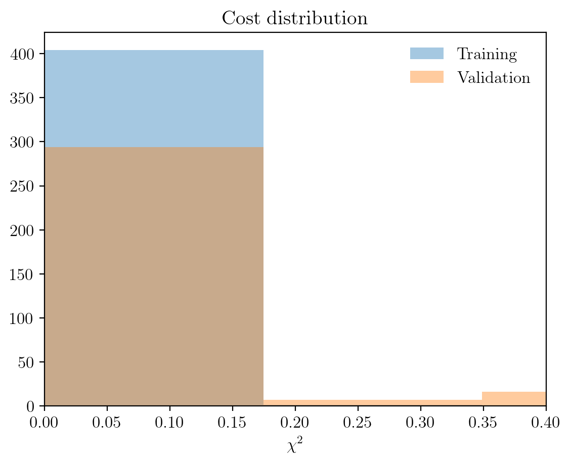
The pretaind models have now been downloaded, so let us see what they look like. The cell immediately below loads the models, plots the cost distribution on the training and validation sets and plots how the predicted ZLPs behave as a function of the total integrated intensity per cluster:
[10]:
im.load_zlp_models(path_to_models=path_to_pretrained_models, based_on='log_zlp', plot_chi2=True, plot_pred=True)
Loading hyper-parameters complete
Loading scale variables for zlp models complete
# of spectra per cluster is [6416 2057  261  132 3166]
Clustering based on cluster centroids complete
Loading models complete
Chi2 plot saved at C:\Users\abelbrokkelkam\OneDrive - Delft University of Technology\PhD\Programming\Python\CBL-ML\sphinx\source\installation\output\
Cluster predictions plot saved at C:\Users\abelbrokkelkam\OneDrive - Delft University of Technology\PhD\Programming\Python\CBL-ML\sphinx\source\installation\output\
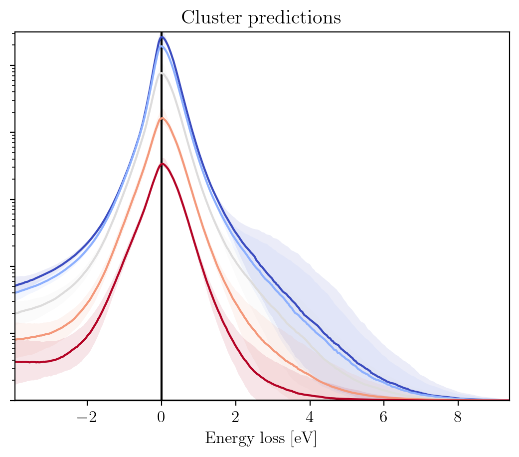
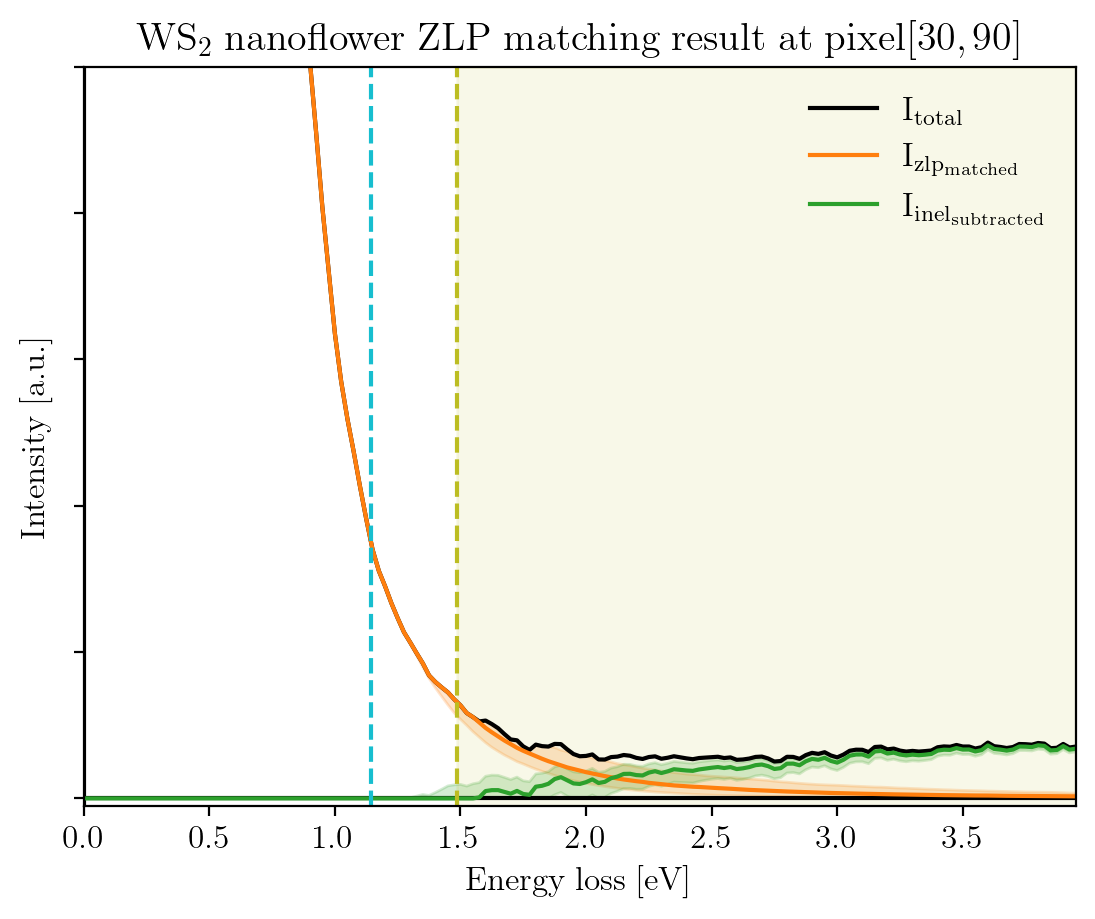
This shows that the clustering has been effective, since the ZLPs do not overlap before \(E_I\). Let us consider a specific pixel, say (30, 90), to see how the subtracted spectrum compares to the raw spectrum.
[11]:
pixx = 30
pixy = 90
signal_type = 'pool'

fig = plot_zlp_per_pixel(im, pixx, pixy, signal_type=signal_type,
                          zlp_gen=False, zlp_match=True,
                          subtract=True, deconv=False,
                          hyper_par=True, random_zlp=None,
                          title=title_specimen + r"$\rm{ZLP\;matching\;result\;at\;pixel[%d,%d]}$" % (pixx, pixy),
                          xlabel=r"$\rm{Energy\;loss\;[eV]}$", ylabel=r"$\rm{Intensity\;[a.u.]}$",
                          xlim=[0, -1*im.eaxis[0]], ylim=[-10, 1e3])
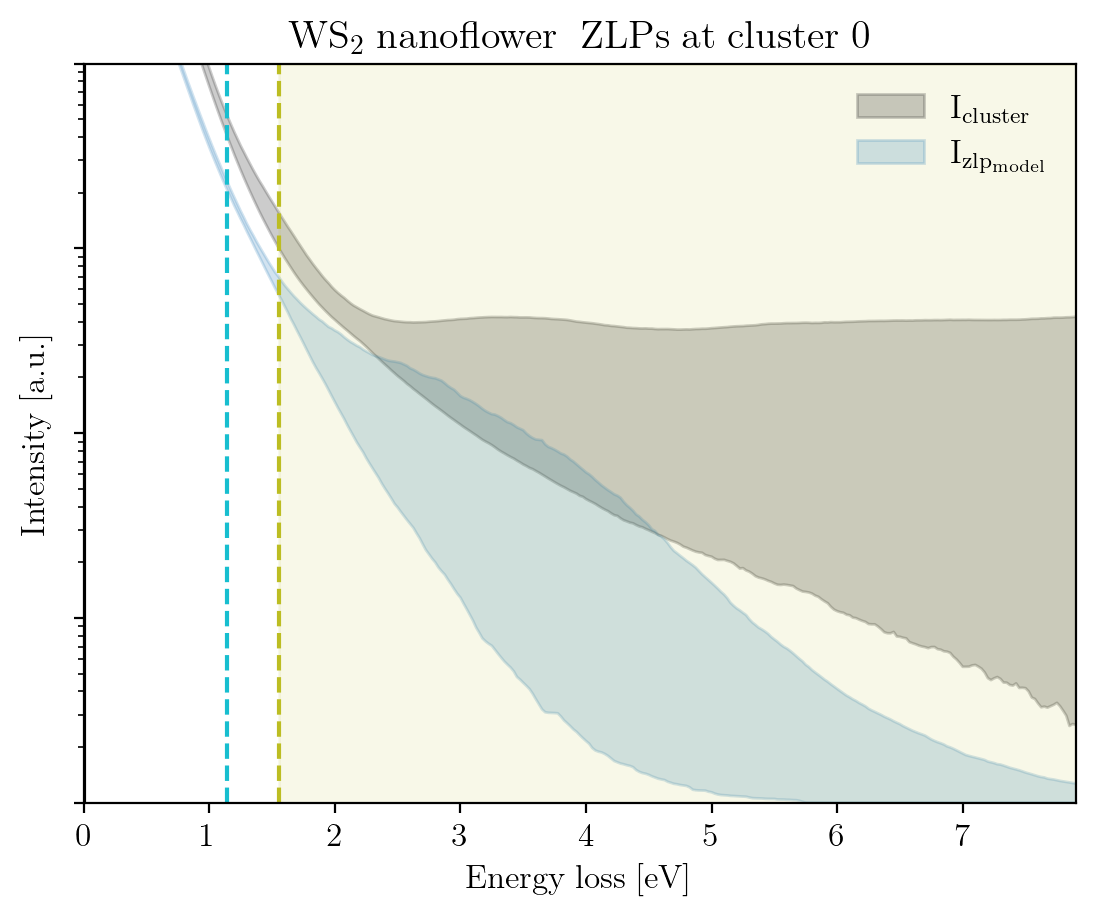
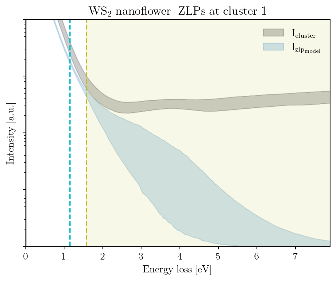
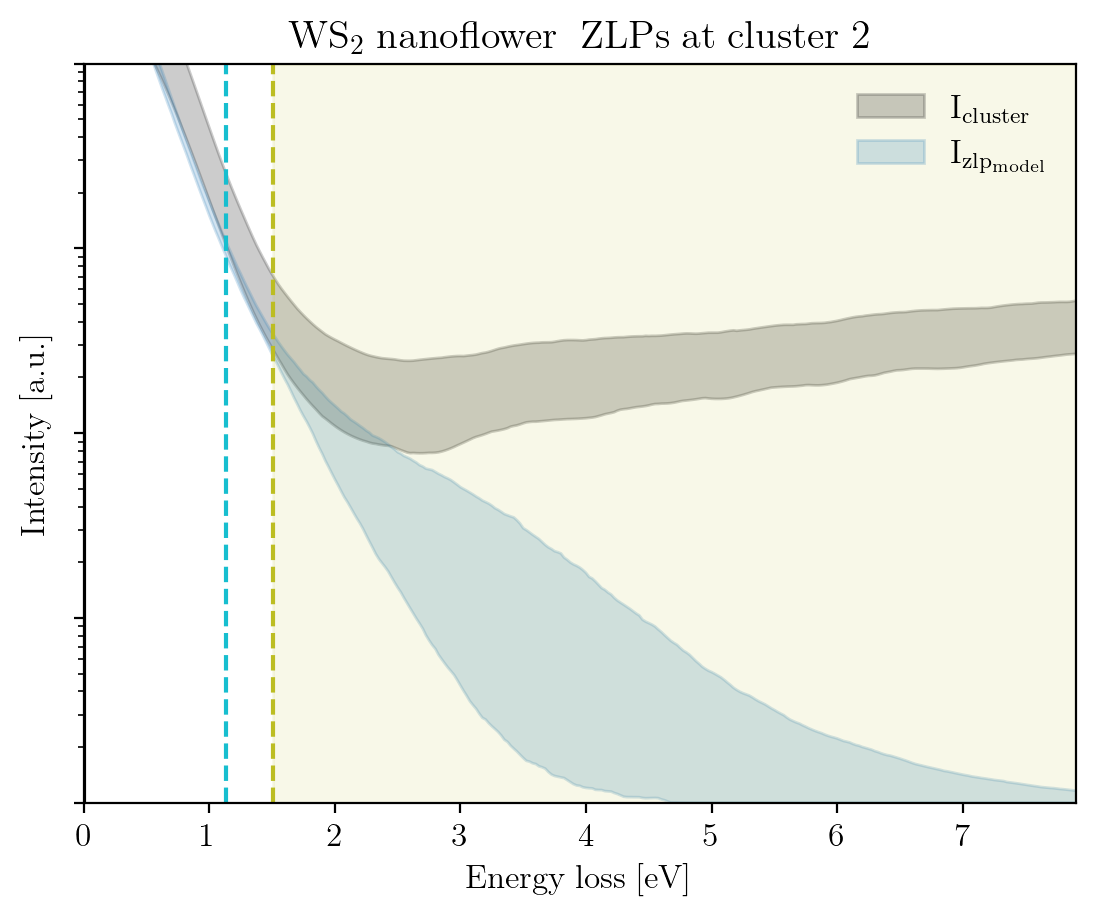
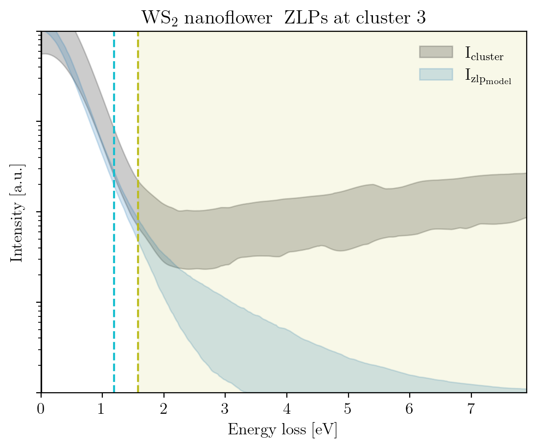
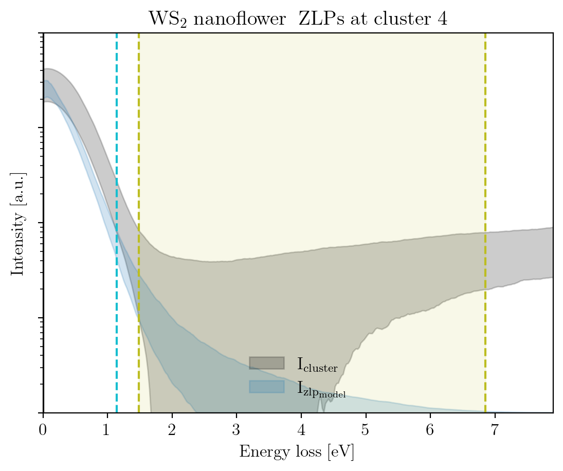
We conclude this tutorial by plotting, for each cluster, the raw signal plus the ZLP with uncertainties evaluated at the cluster means:
[14]:
signal_type = 'EELS'
for cluster, centroid in enumerate(im.cluster_centroids):
    fig = plot_zlp_per_cluster(im, cluster=cluster, signal_type=signal_type,
                               zlp_gen=True, hyper_par=True, smooth=True,
                               title=title_specimen + r"$\rm{\;ZLPs\;at\;cluster\;%d}$" % cluster,
                               xlabel=r"$\rm{Energy\;loss\;[eV]}$", ylabel=r"$\rm{Intensity\;[a.u.]}$",
                               yscale='log',
                               xlim=[0, -2*im.eaxis[0]], ylim=[1, 1e4])
[ ]: