Band gap analysis
One important application of ZLP-subtracted EELS spectra is the determination of the band gap energy and type (direct or indirect) in semiconductor materials. The reason is that the onset of the inelastic scattering intensity provides information on the value of the band gap energy \(E_{\rm bg}\), while its shape for \(E \gtrsim E_{\rm bg}\) is determined by the underlying band structure. Different approaches have been put proposed to evaluate \(E_{\rm bg}\) from subtracted EEL spectra, such as by means of the inflection point of the rising intensity or a linear fit to the maximum positive slope [Schamm and Zanchi, 2003]. Following [Roest et al., 2021], here we adopt the method of [Rafferty and Brown, 1998, Rafferty et al., 2000], where the behaviour of \(I_{\rm inel}(E)\) in the region close to the onset of the inelastic scatterings is described by
and vanishes for \(E < E_{\rm bg}\). Here \(A\) is a normalisation constant, while the exponent \(b\) provides information on the type of band gap: it is expected to be \(b\simeq0.5~(1.5)\) for a semiconductor material characterised by a direct (indirect) band gap. While (37) requires as input the complete inelastic distribution, in practice the onset region is dominated by the single-scattering distribution, since multiple scatterings contribute only at higher energy losses.
The band gap energy \(E_{\rm bg}\), the overall normalisation factor \(A\), and the band gap exponent \(b\) can be determined from a least-squares fit to the experimental data on the ZLP-subtracted spectra. This polynomial fit is carried out in the energy loss region around the band gap energy, \([ E^{(\rm fit)}_{\rm min}, E^{(\rm fit)}_{\rm max}]\). A judicious choice of this interval is necessary to achieve stable results: a too wide energy range will bias the fit by probing regions where Eq. (37) is not necessarily valid, while a too narrow fit range might not contain sufficient information to stabilize the results and be dominated by statistical fluctuation.
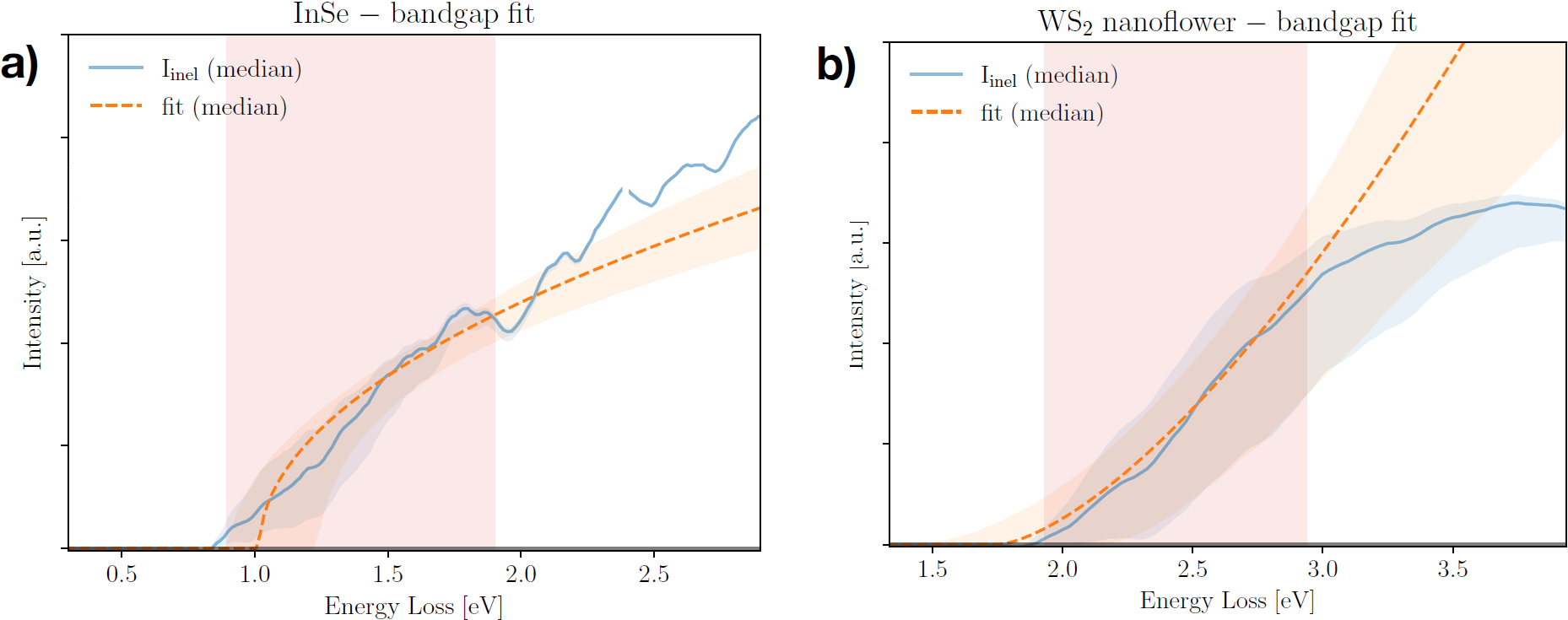
Fig. 6 Representative examples of bandgap fits to the onset of inelastic spectra in the InSe (a) and WS 2 (b) specimens. The red shaded areas indicate the polynomial fitting range, the blue curve and band corresponds to the median and 68% CL intervals of the ZLP-subtracted intensity \(I_{\rm inel}(E)\) , and the outcome of the bandgap fits based on Eq. (37) is indicated by the green dashed curve (median) and band (68% CL intervals).
Fig. 6 (a,b) displays representative examples of bandgap fits to the onset of the inelastic spectra in the InSe (WS2) specimens respectively. The red shaded areas indicate the fitting range, bracketed by \(E^{(\rm fit)}_{\rm min}\) and \(E^{(\rm fit)}_{\rm max}\). The blue curve and band corresponds to the median and 68% CL intervals of the ZLP-subtracted intensity \(I_{\rm inel}(E)\), and the outcome of the band gap fits based on Eq. (37) is indicated by the green dashed curve (median) and band (68% CL intervals). Here the onset exponents \(b\) have been kept fixed to \(b=0.5~(1/5)\) for the InSe (WS2) specimen given the direct (indirect) nature of the underlying band gaps. One observes how the fitted model describes well the behaviour of \(I_{\rm inel}(E)\) in the onset region for both specimens, further confirming the reliability of our strategy to determine the band gap energy \(E_{\rm bg}\). As mentioned in [Rafferty et al., 2000], it is important to avoid taking a too large interval for \([ E^{(\rm fit)}_{\rm min}, E^{(\rm fit)}_{\rm max}]\), else the polynomial approximation ceases to be valid, as one can also see directly from these plots.
Retardation losses
When attempting to measure the band gap using EELS, it is important to consider the effects of retardation losses (or Cerenkov losses) [Stöger-Pollach et al., 2006, Stöger-Pollach, 2008, Horák and Stöger-Pollach, 2015, Erni, 2016]. For more details see: The role of relativistic contributions. In short, the retardation losses can pose a limit on the determination of electronic properties in the low loss region. The best course of action is to reduce the influence of retardation effects (e.g. lower beam voltage, sample thickness considerations) when taking measurements.