ml4eft.analyse.analyse.Analyse#

class ml4eft.analyse.analyse.Analyse(path_to_models, order='quad', all=False)[source]#

Bases: object

Post-training analyser that loads and evaluates models

__init__(path_to_models, order='quad', all=False)[source]#

Analyse constructor

Parameters

path_to_models (dict) – Of the form {‘lin’: {‘c1’: <path_to_c1_models>, ‘c2’: <path_to_c2_models>}, ‘quad’: {‘c1_c1’: <path_to_c1_c1_models>}, {‘c1_c2’: <path_to_c1_c2_models>}, {‘c2_c2’: <path_to_c2_c2_models>}}
order (str, default='quad') – The order in the EFT expansion (choose between either ‘lin’ or ‘quad’)
all (bool, default='True') – When set to True, the analyser loads all replicas. Set to False by defualt, in which case the replicas are clusterd into “good” and “bad” models based on their loss value.

Examples

Trained models can be loaded by creating an ml4eft.analyse.analyse.Analyse object

>>> analyser = Analyse(path_to_models, 'quad')

Followed by constructing a model dictionary that contains all the models plus associated settings

>>> analyser.build_model_dict()
>>> analyser.model_df
                models              idx             scalers                                       run_card              rep_paths
lin  c1         [Classifier() ...   [rep_idx, ...]  [RobustScaler(quantile_range=(5,95)), ...]    {'name': 'c1', ...}   [<path_to_rep>, ...]
     c2         [Classifier() ...   ...             ...                                           ...                   ...
quad c1_c1      [Classifier() ...   ...             ...                                           ...                   ...
     c1_c2      [Classifier() ...   ...             ...                                           ...                   ...
     c2_c2      [Classifier() ...   ...             ...                                           ...                   ...

Events and the inclusive cross-section can be loaded into a DataFrame by

>>> df, xsec = analyser.load_events('.../events_<rep>.pkl.gz')
>>> df
          sqrts_hat       pt_l1       pt_l2  pt_l_leading  pt_l_trailing   ...
1       1702.356400   20.532279  308.295118    308.295118      20.532279   ...
2       ...           ...        ...           ...             ...

To evaluate the models on the loaded DataFrame df, use:

>>> analyser.evaluate_models(df)
>>> analyser.models_evaluated_df['models']
>>> analyser.models_evaluated_df['models']
lin   c1            [[0.05130317, 0.05723376, 0.058220766, 0.04042...
      c2            [[0.074420996, 0.10293982, 0.10705493, 0.05695...
quad  c1_c1         [[0.07958487, 0.13463444, 0.14215767, 0.049889...
      c1_c2         [[0.0005354581, 0.00042073405, 0.0004430262, -...
      c2_c2         [[0.00032746396, 0.00041523552, 0.00045115477,...

Methods

`__init__`(path_to_models[, order, all])	Analyse constructor
`accuracy_heatmap`(c_name, order, process[, ...])	Compares the NN and true EFT ratio functions and plots their ratio and pull
`build_model_dict`([rep, epoch])	Constructs a DataFrame with loaded models plus associated info
`build_path_dict`(root, order, prefix)	Construct path to model dictionary
`coeff_function_truth`(df, c_name, features, ...)	Evaluates the analytic EFT ratio functions \(r_{\sigma}^{(i)}\) and \(r_{\sigma}^{(i,j)}\)
`decision_function_nn`(c[, df, epoch])	Computes the Neural Network parameterised decision function \(g(x, c)\)
`decision_function_truth`(events, c, features, ...)	Computes the analytic decision function
`evaluate_models`(df[, rep, epoch])	Evaluates the loaded models on a Pandas DataFrame `df`
`filter_out_models`(losses)	Filter out the badly trained models based on kmeans clustering.
`get_event_paths`(root_path)	Returns a list of paths to the DataFrames at `root_path`
`likelihood_ratio_nn`(c[, df, epoch])	Compute the Neural Network parameterised likelihood ratio
`likelihood_ratio_truth`(events, c, features, ...)	Computes the analytic likelihood ratio \(r(x, c)\)
`load_events`(event_path)	Loads a event DataFrame and splits it into the events and the inclusive cross section
`load_loss`(path_to_loss)	Loades the losses per epoch into a list
`load_models`(model_path[, rep, epoch])	Loads the trained models
`load_run_card`(path)	Loads training run card
`plot_accuracy_1d`(c, c_name, process, order, ...)	Plots the decision boundary \(g(x,c)\) as predicted by the ML model and the analytical (exact) model along 1 dimension, i.e :x=math:m_{tt}
`plot_heatmap`(ax, data, xlabel, ylabel, ...)	Plot and return a heatmap of `data`
`plot_heatmap_overview`(c_name, order, process)	Produces an overview of heatmaps showing in each plot the ratio between the ML model prediction and the analytical EFT ratio function \(r_{\sigma}^{(i)}\) or \(r_{\sigma}^{(i, j)}\)
`plot_loss_overview`(c_name, order[, ax, rep, ...])	Plots the loss evolution per replica and returns an overview plot
`point_by_point_comp`(df, c_name, c, features, ...)	Produces a point by point comparison overview per replica of the log-likelihood ratio between the ML model and the analytical (exact) model
`point_by_point_comp_med`(df, c, features, ...)	Produces a point by point comparison of the log-likelihood ratio between the (median) ML model and the analytical (exact) model
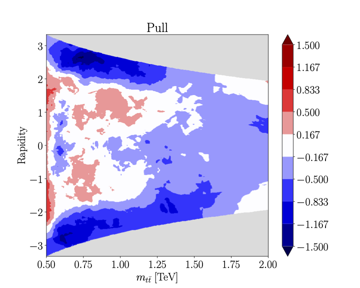
`posterior_loader`(path)	Loads the posterior samples at `path` and converts it to a DataFrame

accuracy_heatmap(c_name, order, process, mx_cut=None, rep=None, epoch=- 1, ax=None, text=None)[source]#

Compares the NN and true EFT ratio functions and plots their ratio and pull

Parameters

c_name (str) – Name of the EFT parameter, e.g. ‘ctgre’
order (str) – Order in the EFT expansion, options are ‘lin’ or ‘quad’
process (str) – Specifies the process. Currently supported is ‘tt’ and ‘ZH’
mx_cut (list, optional) – Plot range of the invariant mass
rep (int, optional) – Request to plot for a specific replica
epoch (int, optional) – Request to plot for a specific epoch.
ax (matplotlib.pyplot.axes, optional) – Axes to plot on
text (str, optional) – Add additional text on the heatmap such as the replica number

Returns

matplotlib.figure.Figure – Heatmap of EFT ratio function
matplotlib.figure.Figure – Heatmap of associated pull

Examples

For a single EFT coefficient \(c_{tG}\) the likelihood ratio takes the form

\[r_{\sigma}(x, c_{tG}) = 1 + c_{tG} r_{\sigma}^{(c_{tG})} + c_{tG}^2 r_{\sigma}^{(c_{tG}, c_{tG})}\]

To plot for example the accuracy of \(r_{\sigma}^{(c_{tG}, c_{tG})}\) by plotting its ratio to the exact result, one runs

>>> fig_med, fig_pull = analyser.accuracy_heatmap('ctgre_ctgre', 'quad', 'tt')
>>> fig_med

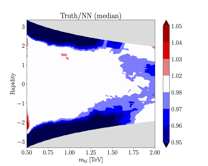
>>> fig_pull

build_model_dict(rep=None, epoch=- 1)[source]#

Constructs a DataFrame with loaded models plus associated info

Parameters

rep (int, optional) – Replica number in case a specific replica is requested
epoch (int, optional) – Epoch to load, set to the best model by default

static build_path_dict(root, order, prefix)[source]#

Construct path to model dictionary

Parameters

root (str) – Path to the model root directory
order (str) – Order of the EFT expansion, choose between ‘lin’ and ‘quad’
prefix (str) – For models: prefix = models, for theory predictions: prefix = ``process_id`

Returns

path_to_models – Dictionary containing the paths to the models for each EFT ratio function

Return type

dict

coeff_function_truth(df, c_name, features, process, order)[source]#

Evaluates the analytic EFT ratio functions \(r_{\sigma}^{(i)}\) and \(r_{\sigma}^{(i,j)}\)

Parameters

df (pandas.DataFrame) – Events on which to evaluate \(r_{\sigma}^{(i)}\) and \(r_{\sigma}^{(i,j)}\)
c_name (str) – Name of the EFT coefficient. Choose between ‘ctgre’, ‘cut’, ‘cut_cut’, ‘ctgre_ctgre’
features (list) – Kinematic features, options are m_tt, y
process (str) – Supported options are ‘tt’ or ‘ZH’
order (str) – Order of the EFT expansion, choose between ‘lin’ and ‘quad’

Returns

coeff – (N,) ndarray with \(r_{\sigma}^{(i)}\) or \(r_{\sigma}^{(i,j)}\) evaluated on df depending on the order

Return type

array_like

decision_function_nn(c, df=None, epoch=- 1)[source]#

Computes the Neural Network parameterised decision function \(g(x, c)\)

Parameters

df (pd.DataFrame) – event info
c (dict) – EFT point
epoch (int, optional) – Use models at a specific epoch, set to -1 (best modeL) by default

Returns

decision_function – NN decision function

Return type

numpy.ndarray

decision_function_truth(events, c, features, process, order=None)[source]#

Computes the analytic decision function

Parameters

order (str, optional) – Specifies the order in the EFT expansion. Must be one of lin, quad.
process (str) – Choose between tt or ZH
features (list) – List of kinematic labels
events (pd.DataFrame) – Pandas DataFrame with the events
c (numpy.ndarray, shape=(M,)) – EFT point in M dimensions, e.g c = (cHW, cHq3)

Returns

decision_function – Truth decision function

Return type

numpy.ndarray

evaluate_models(df, rep=None, epoch=- 1)[source]#

Evaluates the loaded models on a Pandas DataFrame df

Parameters

df (pd.DataFrame) – input to the models
rep (int, optional) – Replica number in case a specific replica is requested. Set to None by default in which case all available replicas are included.
epoch (int, optional) – Epoch number to load. Set to the best model by default.

filter_out_models(losses)[source]#

Filter out the badly trained models based on kmeans clustering.

Parameters: losses (array_like) – Losses of all the trained models
Returns: good_model_idx – Array indices of the ‘good’ models
Return type: numpy.ndarray

static get_event_paths(root_path)[source]#

Returns a list of paths to the DataFrames at root_path

Parameters: root_path (str) – path to the DataFrame directory
Returns: event_paths – list of paths to the DataFrames at stored at root_path
Return type: list

Examples

The paths to the event DataFrames stored at root_path can be loaded for ‘n_rep’ replicas by

>>> analyser.get_event_paths('/training_data/tt_llvlvlbb/tt_c1')
[/training_data/tt_llvlvlbb/tt_c1/events_0.pkl.gz', ... , /training_data/tt_llvlvlbb/tt_c1/events_<n_rep>.pkl.gz']

likelihood_ratio_nn(c, df=None, epoch=- 1)[source]#

Compute the Neural Network parameterised likelihood ratio

Parameters

c (dict) – Of the form {‘c1’: value, ‘c2’: value, …}
df (pandas.DataFrame, optional) – In case the loaded models have not been evaluated yet, one can pass df to evaluate the neural networks
epoch (int, optional) – Specify an epoch if necessary, takes the best model by default

Returns

ratio – likelihood ratio as (N,M) ndarray with N and M the number of replicas and events respectively

Return type

array_like

static likelihood_ratio_truth(events, c, features, process, order=None)[source]#

Computes the analytic likelihood ratio \(r(x, c)\)

Parameters

order (str, optional) – Specifies the order in the EFT expansion. Must be one of lin, quad.
process (str) – Choose between tt or ZH
features (list) – List of kinematic labels
events (pd.DataFrame) – Pandas DataFrame with the events
c (dict) – EFT point with operator names specified as keys

Returns

ratio – Likelihood ratio wrt the SM

Return type

numpy.ndarray

static load_events(event_path)[source]#

Loads a event DataFrame and splits it into the events and the inclusive cross section

Parameters

event_path (str) – Path to the DataFrame (including the xsec as first row)

Returns

events (pandas.DataFrame) – DataFrame with events
xsec (float) – Inclusive cross-section of the events

static load_loss(path_to_loss)[source]#

Loades the losses per epoch into a list

Parameters: path_to_loss (str) – Path to loss file
Returns: loss – list of losses per epoch
Return type: list

load_models(model_path, rep=None, epoch=- 1)[source]#

Loads the trained models

Parameters

model_path (str) – path to model directory
rep (int, optional) – Load only a specific replica specified by rep. Load all replicas by default.
epoch (int, optional) – Model at specific epoch to load. Set to the best model by default.

Returns

models (array_like) – (N,) ndarray containing the loaded neural networks
models_rep_nr (array_like) – (N,) ndarray containing the replica numbers of the loaded neural networks
scalers (array_like) – (N,) ndarray containing the preprocessing scalers of the loaded neural networks
run_card (dict) – training run card of the trained models
rep_paths (array_like) – (N,) ndarray with the paths to the neural networks

static load_run_card(path)[source]#

Loads training run card

Parameters: path (str) – path to json model run card that stores the hyperparameter settings
Returns: run_card – dict with all the hyperparameter settings
Return type: dict

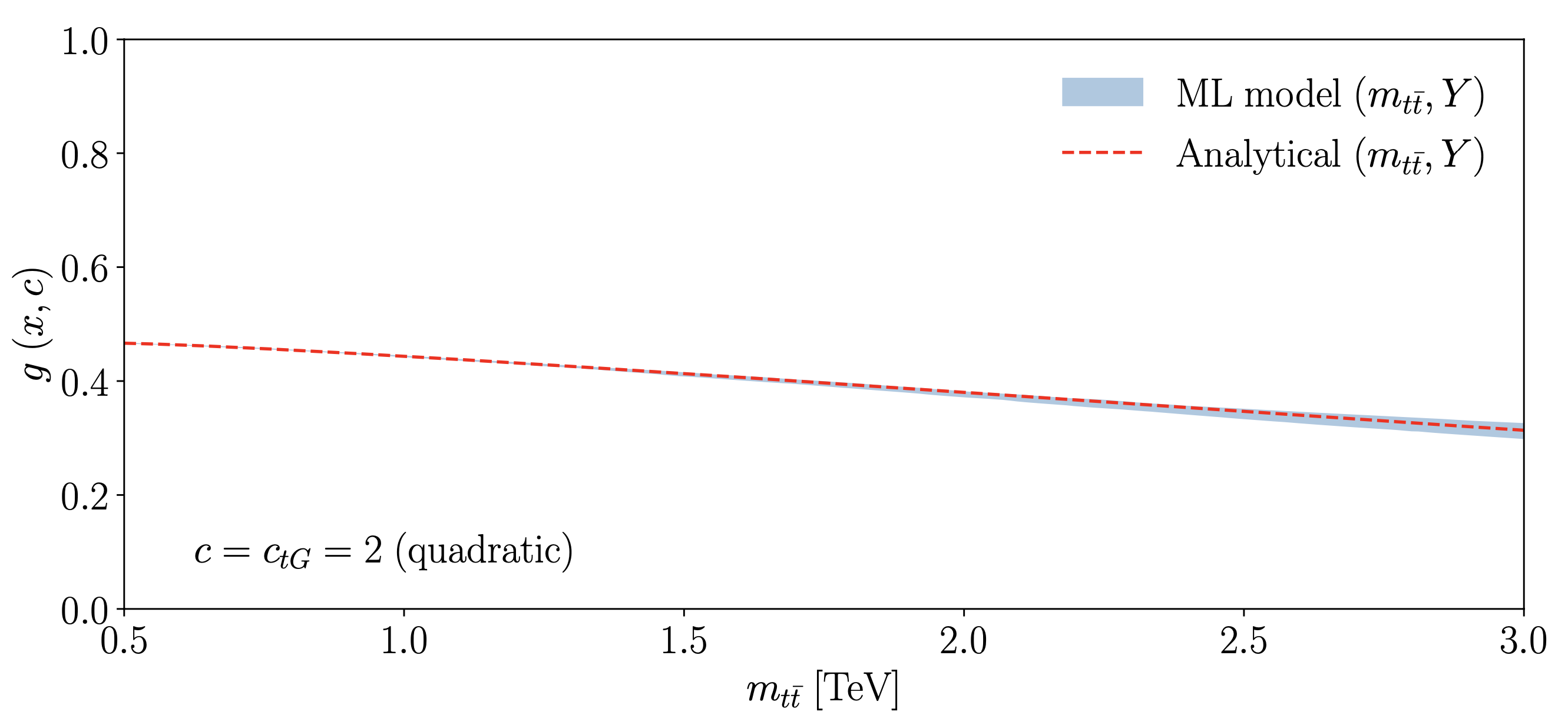
plot_accuracy_1d(c, c_name, process, order, mx_cut, epoch=- 1, ax=None, text=None)[source]#

Plots the decision boundary \(g(x,c)\) as predicted by the ML model and the analytical (exact) model along 1 dimension, i.e :x=math:m_{tt}

Parameters

c (dict) – Of the form {‘c1’: value, ‘c2’: value}
process (str) – Choose between tt or ZH
order (str, optional) – Specifies the order in the EFT expansion. Must be one of lin, quad.
mx_cut (list) – Plot range of the invariant mass
epoch (int, optional) – Specific epoch to plot, set to the best models by default
ax (matplotlib.axes, optional) – Plot on an already created axes object
text (str, optional) – Additional text to show on the plot

Returns

fig – Plot comparing the decision boundary \(g(x,c)\) as predicted by the ML model and the analytical (exact) result

Return type

matplotlib.figure

Examples

>>> analyser = Analyse(path_to_models, 'quad')
>>> fig = analyser.plot_accuracy_1d(c={'ctgre': -2, 'cut': 0}, process='tt', order='quad', cut=0.5, text=r'$c=c_{tG}=2\;\mathrm{quadratic}$')
>>> fig

static plot_heatmap(ax, data, xlabel, ylabel, title, extent, bounds, cmap='GnBu', rep=None, text=None)[source]#

Plot and return a heatmap of data

Parameters

data (numpy.ndarray, shape=(M, N)) – Input array
xlabel (str) – x-label
ylabel (str) – y-label
title (str) – title of plot
extent (list) – boundaries of the heatmap, e.g. [x_0, x_1, y_1, y_2]
bounds (list) – The boundaries of the discrete colourmap
cmap (str) – colourmap to use, set to ‘GnBu’ by default

Returns

fig

Return type

matplotlib.figure.Figure

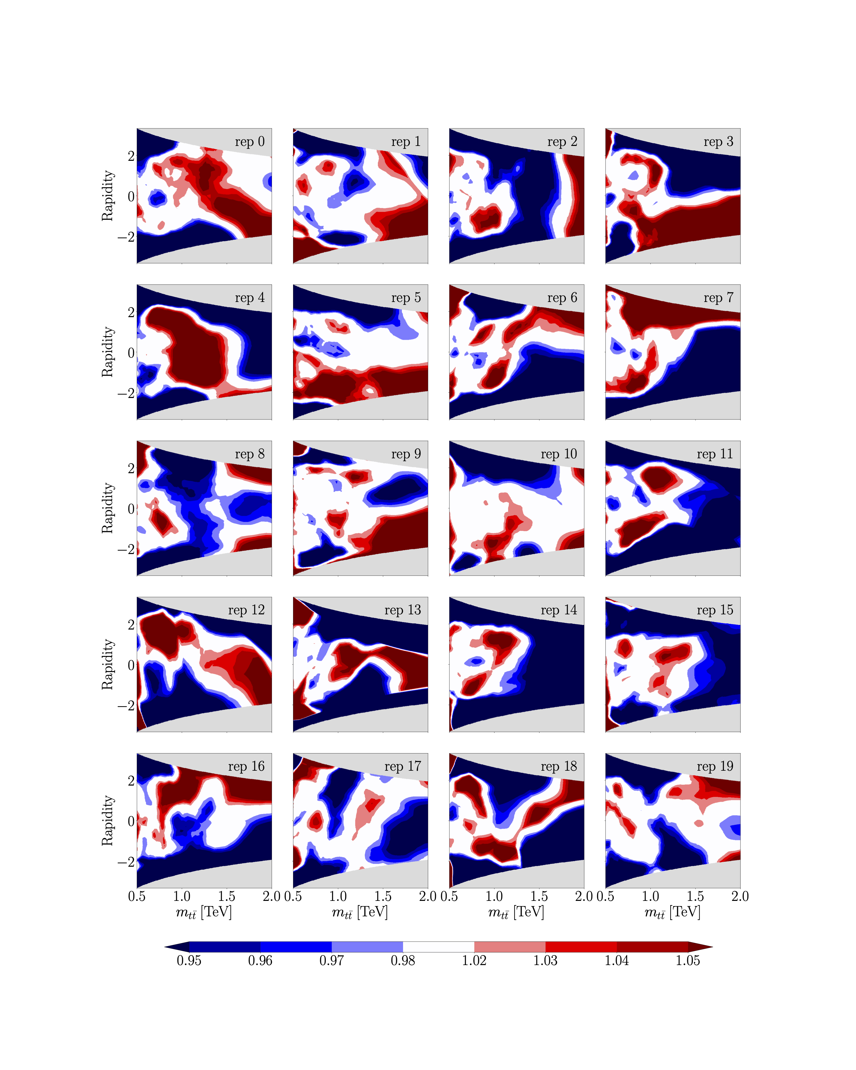
plot_heatmap_overview(c_name, order, process, mx_cut=None, reps=None, epoch=- 1)[source]#

Produces an overview of heatmaps showing in each plot the ratio between the ML model prediction and the analytical EFT ratio function \(r_{\sigma}^{(i)}\) or \(r_{\sigma}^{(i, j)}\)

Parameters

c_name (str) – Name of EFT coefficient
order (str) – Order in the EFT expansion
process (str) – Specifies the process, choose between ‘tt’ and ‘ZH’
mx_cut (float, optional) – Plot range of the invariant mass
reps (int, optional) – Number of replicas to include in the heatmap overview
epoch (int, optional) – Specific epoch to plot at, takes the best models by default

Returns

fig

Return type

matplotlib.figure

Examples

To produce a heatmap overview of the first 20 replicas, run

>>> analyser = Analyse(path_to_models, 'quad')
>>> fig = analyser.plot_heatmap_overview('ctgre_ctgre', 'quad', 'tt', cut=0.5, reps=np.arange(20))
>>> fig

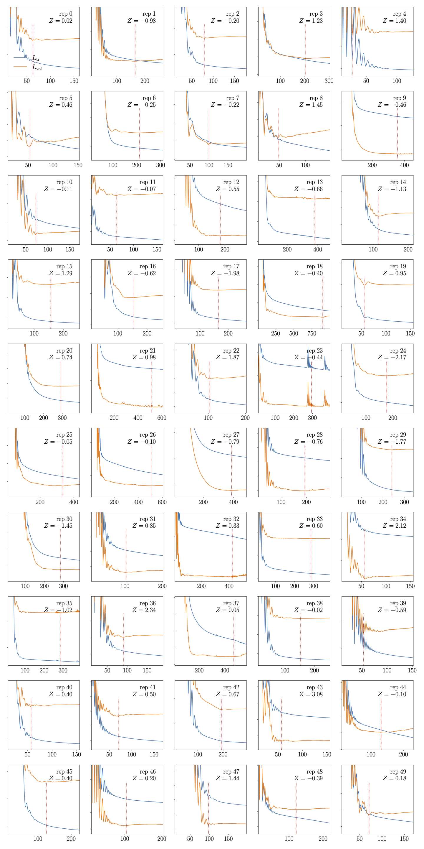
plot_loss_overview(c_name, order, ax=None, rep=None, xlim=None)[source]#

Plots the loss evolution per replica and returns an overview plot

Parameters

c_name (str) – name of EFT parameter
order (str) – Specifies the order in the EFT expansion. Must be one of lin, quad.
ax (matplotlib.axes, optional) – Axes object to plot on
rep (int, optional) – Specific replica to plot

Returns

fig (matplotlib.figure) – Loss overview plot
train_loss_best (array_like) – List of ‘best’ training losses

Examples

To plot a loss overview corresponding to the training of \(r_{\sigma}^{(c_{tG}, c_{tG})}\), run

>>> analyser = Analyse(path_to_models, 'quad')
>>> fig, train_losses = analyser.plot_loss_overview('ctgre_ctgre', 'quad')
>>> fig

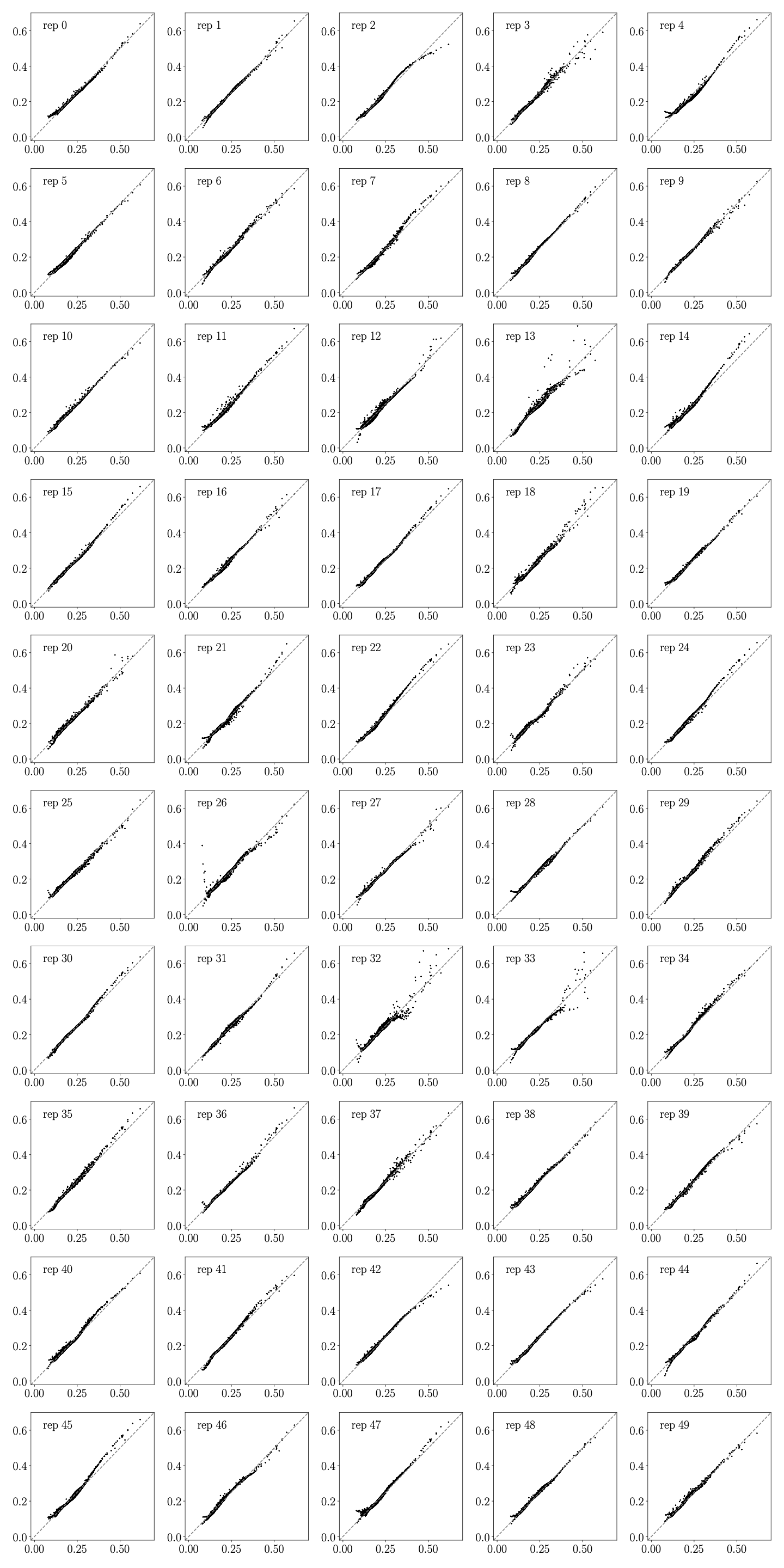
point_by_point_comp(df, c_name, c, features, process, order)[source]#

Produces a point by point comparison overview per replica of the log-likelihood ratio between the ML model and the analytical (exact) model

Parameters

df (pandas.DataFrame) – DataFrame with events
c_name (str) – name of EFT ratio function to compare, e.g. c1_c2
c (dict) – Of the form {‘c1’: value, ‘c2’: value}
features (array_like) – List of features to include in the comparison
process (str) – Choose between tt or ZH
order (str) – Specifies the order in the EFT expansion. Must be one of lin, quad.

Examples

>>> analyser = Analyse(path_to_models, 'quad')
>>> fig, ax = plt.subplots()

>>> events_sm = pd.read_pickle('<events_sm_0.pkl.gz>')
>>> analyser.point_by_point_comp(events_sm, {'ctgre': -2, 'cut': 0}, ['y', 'm_tt'], 'tt', 'lin')
>>> fig

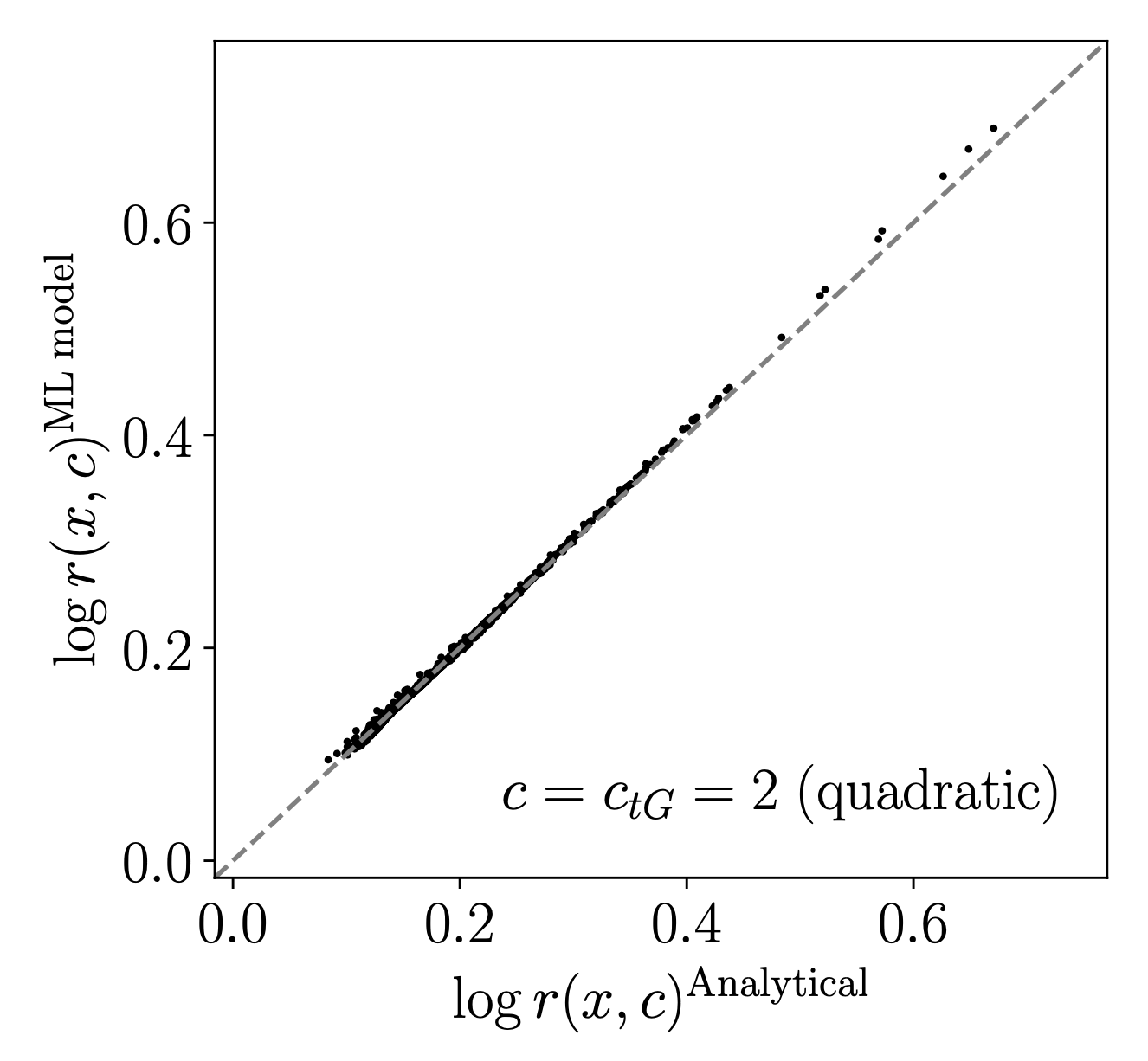
point_by_point_comp_med(df, c, features, process, order, ax, text=None)[source]#

Produces a point by point comparison of the log-likelihood ratio between the (median) ML model and the analytical (exact) model

Parameters

df (pandas.DataFrame) – DataFrame with events
c (dict) – Of the form {‘c1’: value, ‘c2’: value}
features (array_like) – List of features to include in the comparison
process (str) – Choose between tt or ZH
order (str) – Specifies the order in the EFT expansion. Must be one of lin, quad.
ax (matplotlib.axes) – Axes object to plot on
text (str) – Additonal text to put on the plot

Examples

>>> analyser = Analyse(path_to_models, 'quad')
>>> fig, ax = plt.subplots()

>>> events_sm = pd.read_pickle('<events_sm_0.pkl.gz>')
>>> analyser.point_by_point_comp_med(events_sm, {'ctgre': 2, 'cut': 0}, ['y', 'm_tt'], 'tt', 'lin')
>>> fig

static posterior_loader(path)[source]#

Loads the posterior samples at path and converts it to a DataFrame

Parameters: path (str) – Location of posterior samples (.json file)
Returns: df – DataFrame of the posterior samples
Return type: pandas.DataFrame

ML4EFT documentation

ml4eft.analyse.analyse.Analyse

ml4eft.analyse.analyse.Analyse#